引言

本教程將透過一些程式碼演示單應性的基本概念。有關理論的詳細解釋，請參考計算機視覺課程或計算機視覺書籍，例如：

《計算機視覺中的多檢視幾何》(Multiple View Geometry in Computer Vision)，Richard Hartley 和 Andrew Zisserman，[119] （一些章節樣本可在此處獲取，CVPR 教程可在此處獲取）
《三維視覺入門：從影像到幾何模型》(An Invitation to 3-D Vision: From Images to Geometric Models)，Yi Ma, Stefano Soatto, Jana Kosecka, and S. Shankar Sastry，[180] （計算機視覺書籍講義可在此處獲取）
《計算機視覺：演算法與應用》(Computer Vision: Algorithms and Applications)，Richard Szeliski，[263] （電子版可在此處獲取）
《用於視覺控制的單應分解的深入理解》(Deeper understanding of the homography decomposition for vision-based control)，Ezio Malis, Manuel Vargas，[183] （開放訪問可在此處獲取）
《增強現實中的位姿估計：實踐調查》(Pose Estimation for Augmented Reality: A Hands-On Survey)，Eric Marchand, Hideaki Uchiyama, Fabien Spindler，[185] （開放訪問可在此處獲取）

本教程的程式碼可以在C++、Python、Java 找到。本教程中使用的影像可以在此處找到（left*.jpg）。

基本理論

什麼是單應矩陣？

簡而言之，平面單應性關聯了兩個平面之間的變換（直至一個尺度因子）

\[ s \begin{bmatrix} x^{'} \\ y^{'} \\ 1 \end{bmatrix} = \mathbf{H} \begin{bmatrix} x \\ y \\ 1 \end{bmatrix} = \begin{bmatrix} h_{11} & h_{12} & h_{13} \\ h_{21} & h_{22} & h_{23} \\ h_{31} & h_{32} & h_{33} \end{bmatrix} \begin{bmatrix} x \\ y \\ 1 \end{bmatrix} \]

單應矩陣是一個 3x3 矩陣，但具有 8 個自由度（degrees of freedom），因為它是在尺度上進行估計的。它通常透過 \( h_{33} = 1 \) 或 \( h_{11}^2 + h_{12}^2 + h_{13}^2 + h_{21}^2 + h_{22}^2 + h_{23}^2 + h_{31}^2 + h_{32}^2 + h_{33}^2 = 1 \) 進行歸一化（另見 1）。

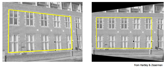
以下示例展示了不同型別的變換，但都關聯了兩個平面之間的變換。

一個平面和影像平面（影像摘自 2）

由兩個相機位置觀察到的平面（影像摘自 3 和 2）

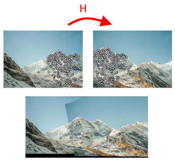
相機繞其投影軸旋轉，等效於認為點位於無窮遠平面上（影像摘自 2）

單應變換有何用處？

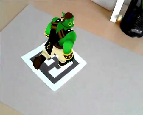
例如，透過標記從共麵點進行增強現實中的相機位姿估計（參見前面的第一個示例）

透視消除/校正（參見前面的第二個示例）

全景影像拼接（參見前面的第二個和第三個示例）

演示程式碼

演示1：從共麵點進行位姿估計

注意: 請注意，從單應性估計相機位姿的程式碼只是一個示例，如果您想估計平面或任意物體的相機位姿，應該使用 cv::solvePnP。

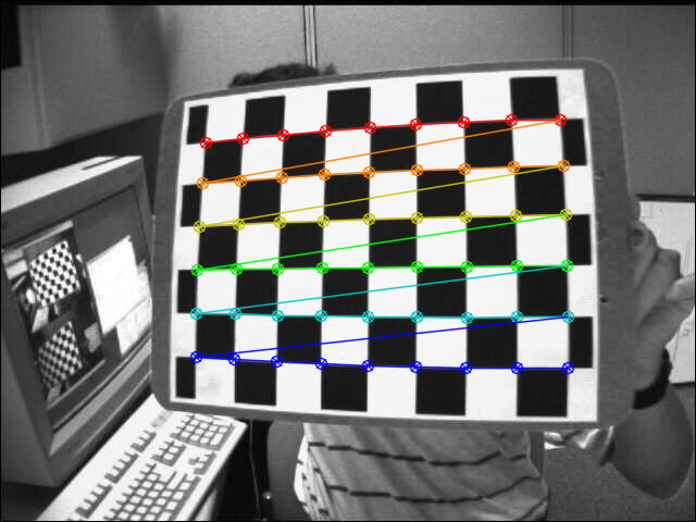
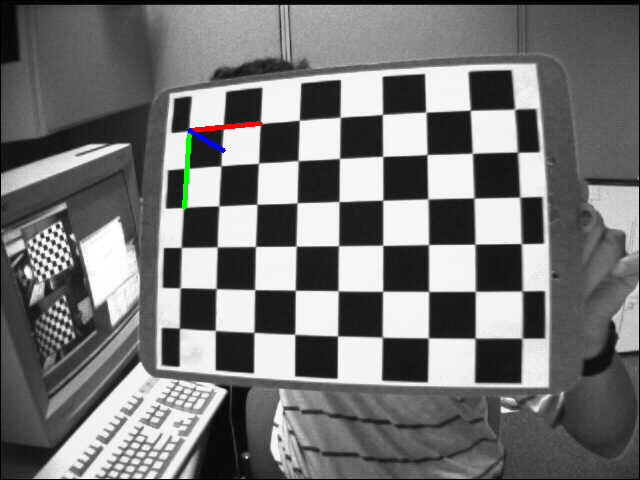
單應性可以使用例如直接線性變換（DLT）演算法進行估計（更多資訊請參見 1）。由於物體是平面的，因此在物體座標系中表示的點與在歸一化相機座標系中表示的投影到影像平面上的點之間的變換是單應性。僅當物體是平面時，才能從單應性中恢復相機位姿，前提是相機內參已知（參見 2 或 4）。這可以透過使用棋盤格物體和 findChessboardCorners() 函式輕鬆測試，以獲取影像中的角點位置。

首先是檢測棋盤格角點，需要棋盤格大小（patternSize），這裡是 9x6

vector<Point2f> corners;

bool found = findChessboardCorners(img, patternSize, corners);

已知棋盤格方塊的大小，可以輕鬆計算在物體座標系中表示的物體點

        for( int i = 0; i < boardSize.height; i++ )
            for( int j = 0; j < boardSize.width; j++ )
corners.push_back(Point3f(float(j*squareSize),
                                          float(i*squareSize), 0));

在單應性估計部分必須移除 Z=0 座標

vector<Point3f> objectPoints;
calcChessboardCorners(patternSize, squareSize, objectPoints);
vector<Point2f> objectPointsPlanar;
    for (size_t i = 0; i < objectPoints.size(); i++)
    {
objectPointsPlanar.push_back(Point2f(objectPoints[i].x, objectPoints[i].y));
    }

歸一化相機中的影像點可以透過角點並應用使用相機內參和畸變係數的反透視變換來計算

    FileStorage fs( samples::findFile( intrinsicsPath ), FileStorage::READ);
    Mat cameraMatrix, distCoeffs;
fs["camera_matrix"] >> cameraMatrix;
fs["distortion_coefficients"] >> distCoeffs;

vector<Point2f> imagePoints;

undistortPoints(corners, imagePoints, cameraMatrix, distCoeffs);

然後可以使用以下方法估計單應性

Mat H = findHomography(objectPointsPlanar, imagePoints);

cout << "H:\n" << H << endl;

從單應矩陣中檢索位姿的快速解決方案是（參見 5）

    // Normalization to ensure that ||c1|| = 1
    double norm = sqrt(H.at<double>(0,0)*H.at<double>(0,0) +
H.at<double>(1,0)*H.at<double>(1,0) +
H.at<double>(2,0)*H.at<double>(2,0));
 
H /= norm;
    Mat c1 = H.col(0);
    Mat c2 = H.col(1);
    Mat c3 = c1.cross(c2);
 
    Mat tvec = H.col(2);
    Mat R(3, 3, CV_64F);
 
    for (int i = 0; i < 3; i++)
    {
R.at<double>(i,0) = c1.at<double>(i,0);
R.at<double>(i,1) = c2.at<double>(i,0);
R.at<double>(i,2) = c3.at<double>(i,0);
    }

\[ \begin{align*} \mathbf{X} &= \left( X, Y, 0, 1 \right ) \\ \mathbf{x} &= \mathbf{P}\mathbf{X} \\ &= \mathbf{K} \left[ \mathbf{r_1} \hspace{0.5em} \mathbf{r_2} \hspace{0.5em} \mathbf{r_3} \hspace{0.5em} \mathbf{t} \right ] \begin{pmatrix} X \\ Y \\ 0 \\ 1 \end{pmatrix} \\ &= \mathbf{K} \left[ \mathbf{r_1} \hspace{0.5em} \mathbf{r_2} \hspace{0.5em} \mathbf{t} \right ] \begin{pmatrix} X \\ Y \\ 1 \end{pmatrix} \\ &= \mathbf{H} \begin{pmatrix} X \\ Y \\ 1 \end{pmatrix} \end{align*} \]

\[ \begin{align*} \mathbf{H} &= \lambda \mathbf{K} \left[ \mathbf{r_1} \hspace{0.5em} \mathbf{r_2} \hspace{0.5em} \mathbf{t} \right ] \\ \mathbf{K}^{-1} \mathbf{H} &= \lambda \left[ \mathbf{r_1} \hspace{0.5em} \mathbf{r_2} \hspace{0.5em} \mathbf{t} \right ] \\ \mathbf{P} &= \mathbf{K} \left[ \mathbf{r_1} \hspace{0.5em} \mathbf{r_2} \hspace{0.5em} \left( \mathbf{r_1} \times \mathbf{r_2} \right ) \hspace{0.5em} \mathbf{t} \right ] \end{align*} \]

這是一個快速解決方案（另見 2），因為它不能確保結果旋轉矩陣是正交的，並且尺度透過將第一列歸一化為 1 來粗略估計。

獲得一個適當的旋轉矩陣（具有旋轉矩陣的特性）的解決方案是應用極分解，或對旋轉矩陣進行正交化（有關資訊請參見 6 或 7 或 8 或 9）

cout << "R (before polar decomposition):\n" << R << "\ndet(R): " << determinant(R) << endl;
    Mat_<double> W, U, Vt;
    SVDecomp(R, W, U, Vt);
R = U*Vt;
    double det = determinant(R);
    if (det < 0)
    {
Vt.at<double>(2,0) *= -1;
Vt.at<double>(2,1) *= -1;
Vt.at<double>(2,2) *= -1;
 
R = U*Vt;
    }
cout << "R (after polar decomposition):\n" << R << "\ndet(R): " << determinant(R) << endl;

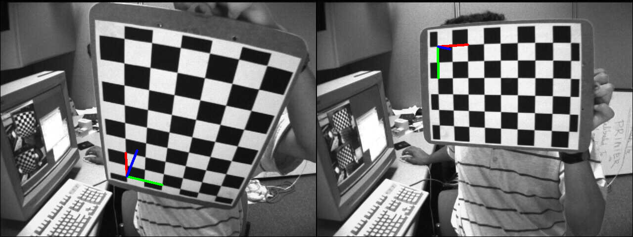
為檢查結果，顯示了使用估計的相機位姿投影到影像中的物體座標系

演示2：透視校正

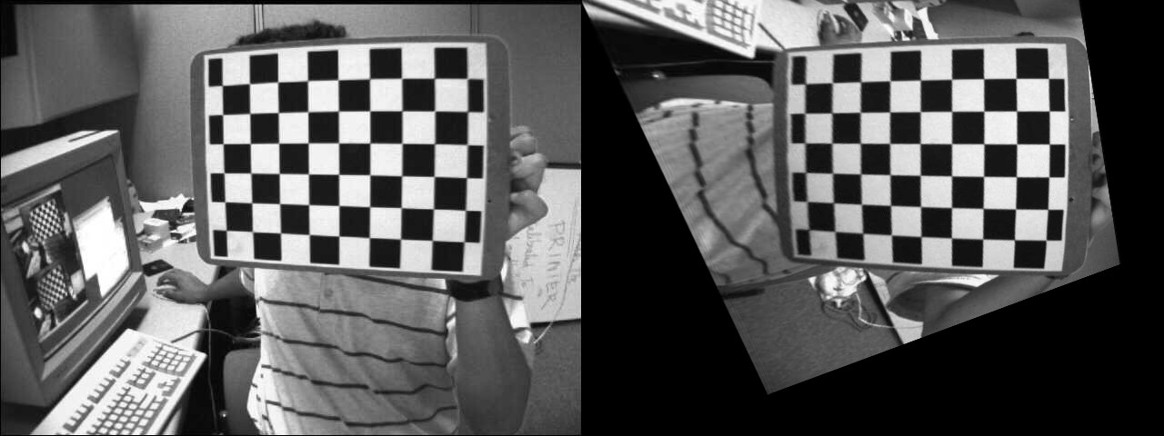
在此示例中，透過計算將源點對映到目標點的單應性，將源影像轉換為所需的透視檢視。下圖顯示了源影像（左）和我們想要轉換為目標棋盤檢視的棋盤檢視（右）。

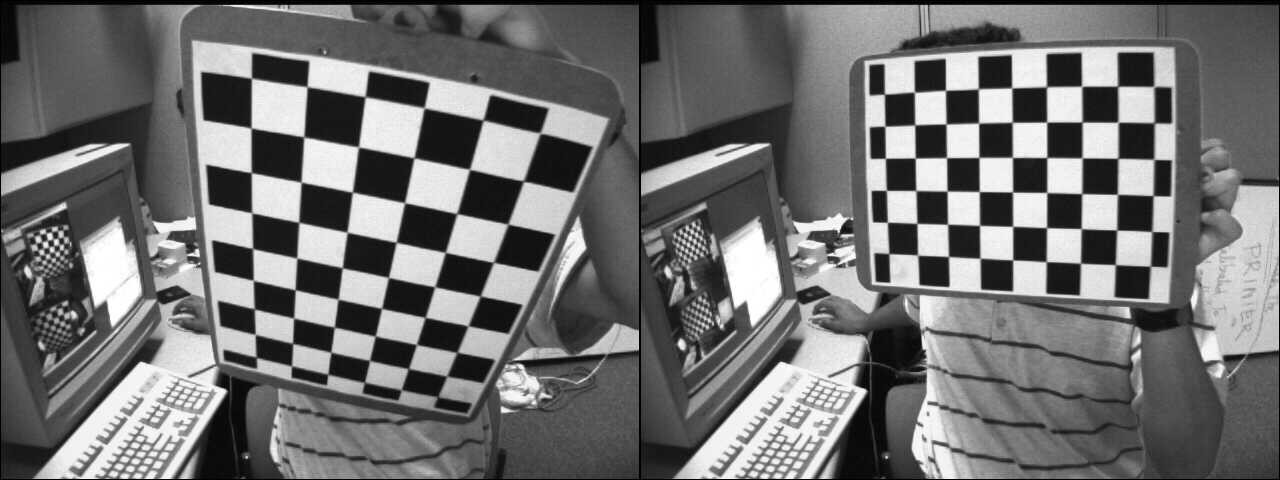
源檢視和目標檢視

第一步是在源影像和目標影像中檢測棋盤格角點

單應性可以輕鬆估計

為了將源棋盤檢視扭曲到目標棋盤檢視，我們使用 cv::warpPerspective

結果影像是

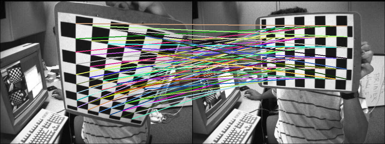
計算透過單應性變換的源角點座標

為了檢查計算的正確性，顯示了匹配線

演示3：從相機位移計算單應

單應性關聯了兩個平面之間的變換，並且可以檢索相應的相機位移，該位移允許從第一個平面檢視轉換到第二個平面檢視（更多資訊請參見 [183]）。在深入探討如何從相機位移計算單應性的細節之前，先回顧一下相機位姿和齊次變換。

函式 cv::solvePnP 允許從對應的 3D 物體點（在物體座標系中表示的點）和投影的 2D 影像點（在影像中觀察到的物體點）計算相機位姿。需要內參和畸變係數（參見相機標定過程）。

\[ \begin{align*} s \begin{bmatrix} u \\ v \\ 1 \end{bmatrix} &= \begin{bmatrix} f_x & 0 & c_x \\ 0 & f_y & c_y \\ 0 & 0 & 1 \end{bmatrix} \begin{bmatrix} r_{11} & r_{12} & r_{13} & t_x \\ r_{21} & r_{22} & r_{23} & t_y \\ r_{31} & r_{32} & r_{33} & t_z \end{bmatrix} \begin{bmatrix} X_o \\ Y_o \\ Z_o \\ 1 \end{bmatrix} \\ &= \mathbf{K} \hspace{0.2em} ^{c}\mathbf{M}_o \begin{bmatrix} X_o \\ Y_o \\ Z_o \\ 1 \end{bmatrix} \end{align*} \]

\( \mathbf{K} \) 是內參矩陣，\( ^{c}\mathbf{M}_o \) 是相機位姿。cv::solvePnP 的輸出正是如此：rvec 是羅德里格斯旋轉向量，tvec 是平移向量。

\( ^{c}\mathbf{M}_o \) 可以用齊次形式表示，並允許將物體座標系中表示的點變換到相機座標系中

\[ \begin{align*} \begin{bmatrix} X_c \\ Y_c \\ Z_c \\ 1 \end{bmatrix} &= \hspace{0.2em} ^{c}\mathbf{M}_o \begin{bmatrix} X_o \\ Y_o \\ Z_o \\ 1 \end{bmatrix} \\ &= \begin{bmatrix} ^{c}\mathbf{R}_o & ^{c}\mathbf{t}_o \\ 0_{1\times3} & 1 \end{bmatrix} \begin{bmatrix} X_o \\ Y_o \\ Z_o \\ 1 \end{bmatrix} \\ &= \begin{bmatrix} r_{11} & r_{12} & r_{13} & t_x \\ r_{21} & r_{22} & r_{23} & t_y \\ r_{31} & r_{32} & r_{33} & t_z \\ 0 & 0 & 0 & 1 \end{bmatrix} \begin{bmatrix} X_o \\ Y_o \\ Z_o \\ 1 \end{bmatrix} \end{align*} \]

將一個座標系中表示的點變換到另一個座標系中可以很容易地透過矩陣乘法完成

\( ^{c_1}\mathbf{M}_o \) 是相機 1 的相機位姿
\( ^{c_2}\mathbf{M}_o \) 是相機 2 的相機位姿

要將相機 1 座標系中表示的 3D 點變換到相機 2 座標系中

\[ ^{c_2}\mathbf{M}_{c_1} = \hspace{0.2em} ^{c_2}\mathbf{M}_{o} \cdot \hspace{0.1em} ^{o}\mathbf{M}_{c_1} = \hspace{0.2em} ^{c_2}\mathbf{M}_{o} \cdot \hspace{0.1em} \left( ^{c_1}\mathbf{M}_{o} \right )^{-1} = \begin{bmatrix} ^{c_2}\mathbf{R}_{o} & ^{c_2}\mathbf{t}_{o} \\ 0_{3 \times 1} & 1 \end{bmatrix} \cdot \begin{bmatrix} ^{c_1}\mathbf{R}_{o}^T & - \hspace{0.2em} ^{c_1}\mathbf{R}_{o}^T \cdot \hspace{0.2em} ^{c_1}\mathbf{t}_{o} \\ 0_{1 \times 3} & 1 \end{bmatrix} \]

在此示例中，我們將計算相對於棋盤格物體，兩個相機位姿之間的相機位移。第一步是計算兩幅影像的相機位姿

vector<Point2f> corners1, corners2;
    bool found1 = findChessboardCorners(img1, patternSize, corners1);
    bool found2 = findChessboardCorners(img2, patternSize, corners2);
 
    if (!found1 || !found2)
    {
cout << "Error, cannot find the chessboard corners in both images." << endl;
        return;
    }
 
vector<Point3f> objectPoints;
calcChessboardCorners(patternSize, squareSize, objectPoints);
 
    FileStorage fs( samples::findFile( intrinsicsPath ), FileStorage::READ);
    Mat cameraMatrix, distCoeffs;
fs["camera_matrix"] >> cameraMatrix;
fs["distortion_coefficients"] >> distCoeffs;
 
    Mat rvec1, tvec1;
    solvePnP(objectPoints, corners1, cameraMatrix, distCoeffs, rvec1, tvec1);
    Mat rvec2, tvec2;
    solvePnP(objectPoints, corners2, cameraMatrix, distCoeffs, rvec2, tvec2);

相機位移可以使用上述公式從相機位姿計算得出

void computeC2MC1(const Mat &R1, const Mat &tvec1, const Mat &R2, const Mat &tvec2,
                  Mat &R_1to2, Mat &tvec_1to2)
{
    //c2Mc1 = c2Mo * oMc1 = c2Mo * c1Mo.inv()
R_1to2 = R2 * R1.t();
tvec_1to2 = R2 * (-R1.t()*tvec1) + tvec2;
}

從相機位移計算出的與特定平面相關的單應性是

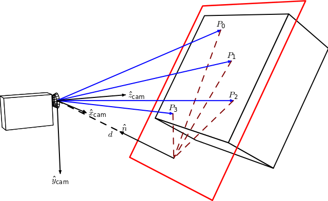
圖片來源：Homography-transl.svg：Per Rosengren 衍生作品：Appoose (Homography-transl.svg) [CC BY 3.0 (http://creativecommons.org/licenses/by/3.0)]，透過維基共享資源

在此圖中，n 是平面的法向量，d 是相機座標系與平面沿平面法線方向的距離。從相機位移計算單應性的方程是

\[ ^{2}\mathbf{H}_{1} = \hspace{0.2em} ^{2}\mathbf{R}_{1} - \hspace{0.1em} \frac{^{2}\mathbf{t}_{1} \cdot \hspace{0.1em} ^{1}\mathbf{n}^\top}{^1d} \]

其中 \( ^{2}\mathbf{H}_{1} \) 是將第一個相機座標系中的點對映到第二個相機座標系中對應點的單應矩陣，\( ^{2}\mathbf{R}_{1} = \hspace{0.2em} ^{c_2}\mathbf{R}_{o} \cdot \hspace{0.1em} ^{c_1}\mathbf{R}_{o}^{\top} \) 是表示兩個相機座標系之間旋轉的旋轉矩陣，而 \( ^{2}\mathbf{t}_{1} = \hspace{0.2em} ^{c_2}\mathbf{R}_{o} \cdot \left( - \hspace{0.1em} ^{c_1}\mathbf{R}_{o}^{\top} \cdot \hspace{0.1em} ^{c_1}\mathbf{t}_{o} \right ) + \hspace{0.1em} ^{c_2}\mathbf{t}_{o} \) 是兩個相機座標系之間的平移向量。

這裡的法向量 n 是在相機座標系 1 中表示的平面法線，可以計算為 2 個向量的叉積（使用平面上的 3 個不共線點），或者在我們的例子中直接使用

Mat normal = (Mat_<double>(3,1) << 0, 0, 1);

Mat normal1 = R1*normal;

距離 d 可以計算為平面法線與平面上一點的點積，或者透過計算平面方程並使用 D 係數

    Mat origin(3, 1, CV_64F, Scalar(0));
    Mat origin1 = R1*origin + tvec1;
    double d_inv1 = 1.0 / normal1.dot(origin1);

投影單應矩陣 \( \textbf{G} \) 可以使用內參矩陣 \( \textbf{K} \) 從歐幾里得單應性 \( \textbf{H} \) 計算得出（參見 [183]），這裡假設兩個平面檢視之間使用相同的相機

\[ \textbf{G} = \gamma \textbf{K} \textbf{H} \textbf{K}^{-1} \]

Mat computeHomography(const Mat &R_1to2, const Mat &tvec_1to2, const double d_inv, const Mat &normal)
{
    Mat homography = R_1to2 + d_inv * tvec_1to2*normal.t();
    return homography;
}

在我們的例子中，棋盤格的 Z 軸指向物體內部，而在單應圖例中它指向外部。這只是一個符號問題

\[ ^{2}\mathbf{H}_{1} = \hspace{0.2em} ^{2}\mathbf{R}_{1} + \hspace{0.1em} \frac{^{2}\mathbf{t}_{1} \cdot \hspace{0.1em} ^{1}\mathbf{n}^\top}{^1d} \]

    Mat homography_euclidean = computeHomography(R_1to2, t_1to2, d_inv1, normal1);
    Mat homography = cameraMatrix * homography_euclidean * cameraMatrix.inv();
 
homography /= homography.at<double>(2,2);
homography_euclidean /= homography_euclidean.at<double>(2,2);

我們現在將比較從相機位移計算的投影單應性與使用 cv::findHomography 估計的單應性。

findHomography H
[0.32903393332201, -1.244138808862929, 536.4769088231476;
 0.6969763913334046, -0.08935909072571542, -80.34068504082403;
 0.00040511729592961, -0.001079740100565013, 0.9999999999999999]
 
從相機位移計算的單應性
[0.4160569997384721, -1.306889006892538, 553.7055461075881;
 0.7917584252773352, -0.06341244158456338, -108.2770029401219;
 0.0005926357240956578, -0.001020651672127799, 1]

單應矩陣相似。如果我們比較使用兩個單應矩陣扭曲的影像 1

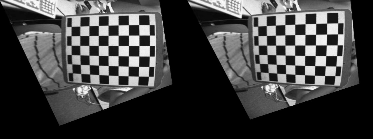
左：使用估計單應性扭曲的影像。右：使用從相機位移計算的單應性。

從視覺上看，很難區分從相機位移計算的單應性與使用 cv::findHomography 函式估計的單應性所產生的影像差異。

練習

這個演示展示瞭如何從兩個相機位姿計算單應變換。嘗試執行相同的操作，但這次計算 N 箇中間單應性。不要計算一個單應性直接將源影像扭曲到所需的相機視點，而是執行 N 次扭曲操作以檢視不同的變換效果。

您應該得到類似以下的結果

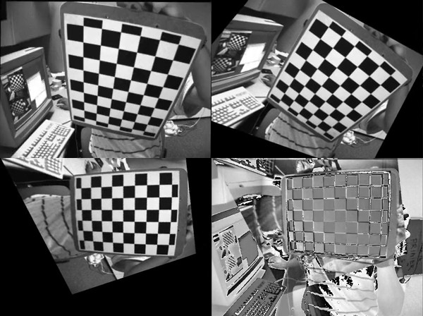
前三幅影像顯示了源影像在三個不同的插值相機視點處被扭曲。第四幅影像顯示了在最終相機視點處扭曲的源影像與目標影像之間的“誤差影像”。

演示4：分解單應矩陣

OpenCV 3 包含了函式 cv::decomposeHomographyMat，它允許將單應矩陣分解為一組旋轉、平移和平面法線。首先，我們將分解從相機位移計算的單應矩陣

    Mat homography_euclidean = computeHomography(R_1to2, t_1to2, d_inv1, normal1);
    Mat homography = cameraMatrix * homography_euclidean * cameraMatrix.inv();
 
homography /= homography.at<double>(2,2);
homography_euclidean /= homography_euclidean.at<double>(2,2);

cv::decomposeHomographyMat 的結果是

vector<Mat> Rs_decomp, ts_decomp, normals_decomp;
    int solutions = decomposeHomographyMat(homography, cameraMatrix, Rs_decomp, ts_decomp, normals_decomp);
cout << "Decompose homography matrix computed from the camera displacement:" << endl << endl;
    for (int i = 0; i < solutions; i++)
    {
      double factor_d1 = 1.0 / d_inv1;
      Mat rvec_decomp;
      Rodrigues(Rs_decomp[i], rvec_decomp);
cout << "Solution " << i << ":" << endl;
cout << "rvec from homography decomposition: " << rvec_decomp.t() << endl;
cout << "rvec from camera displacement: " << rvec_1to2.t() << endl;
cout << "tvec from homography decomposition: " << ts_decomp[i].t() << " and scaled by d: " << factor_d1 * ts_decomp[i].t() << endl;
cout << "tvec from camera displacement: " << t_1to2.t() << endl;
cout << "plane normal from homography decomposition: " << normals_decomp[i].t() << endl;
cout << "plane normal at camera 1 pose: " << normal1.t() << endl << endl;
    }

Solution 0
rvec from homography decomposition: [-0.0919829920641369, -0.5372581036567992, 1.310868863540717]
rvec from camera displacement: [-0.09198299206413783, -0.5372581036567995, 1.310868863540717]
tvec from homography decomposition: [-0.7747961019053186, -0.02751124463434032, -0.6791980037590677] and scaled by d: [-0.1578091561210742, -0.005603443652993778, -0.1383378976078466]
tvec from camera displacement: [0.1578091561210745, 0.005603443652993617, 0.1383378976078466]
plane normal from homography decomposition: [-0.1973513139420648, 0.6283451996579074, -0.7524857267431757]
plane normal at camera 1 pose: [0.1973513139420654, -0.6283451996579068, 0.752485726743176]
 
Solution 1
rvec from homography decomposition: [-0.0919829920641369, -0.5372581036567992, 1.310868863540717]
rvec from camera displacement: [-0.09198299206413783, -0.5372581036567995, 1.310868863540717]
tvec from homography decomposition: [0.7747961019053186, 0.02751124463434032, 0.6791980037590677] and scaled by d: [0.1578091561210742, 0.005603443652993778, 0.1383378976078466]
tvec from camera displacement: [0.1578091561210745, 0.005603443652993617, 0.1383378976078466]
plane normal from homography decomposition: [0.1973513139420648, -0.6283451996579074, 0.7524857267431757]
plane normal at camera 1 pose: [0.1973513139420654, -0.6283451996579068, 0.752485726743176]
 
Solution 2
rvec from homography decomposition: [0.1053487907109967, -0.1561929144786397, 1.401356552358475]
rvec from camera displacement: [-0.09198299206413783, -0.5372581036567995, 1.310868863540717]
tvec from homography decomposition: [-0.4666552552894618, 0.1050032934770042, -0.913007654671646] and scaled by d: [-0.0950475510338766, 0.02138689274867372, -0.1859598508065552]
tvec from camera displacement: [0.1578091561210745, 0.005603443652993617, 0.1383378976078466]
plane normal from homography decomposition: [-0.3131715472900788, 0.8421206145721947, -0.4390403768225507]
plane normal at camera 1 pose: [0.1973513139420654, -0.6283451996579068, 0.752485726743176]
 
Solution 3
rvec from homography decomposition: [0.1053487907109967, -0.1561929144786397, 1.401356552358475]
rvec from camera displacement: [-0.09198299206413783, -0.5372581036567995, 1.310868863540717]
tvec from homography decomposition: [0.4666552552894618, -0.1050032934770042, 0.913007654671646] and scaled by d: [0.0950475510338766, -0.02138689274867372, 0.1859598508065552]
tvec from camera displacement: [0.1578091561210745, 0.005603443652993617, 0.1383378976078466]
plane normal from homography decomposition: [0.3131715472900788, -0.8421206145721947, 0.4390403768225507]
plane normal at camera 1 pose: [0.1973513139420654, -0.6283451996579068, 0.752485726743176]

單應矩陣分解的結果只能恢復到一個尺度因子，該尺度因子實際上對應於距離 d，因為法線是單位長度。正如您所看到的，有一個解決方案與計算出的相機位移幾乎完美匹配。正如文件中所述

如果透過應用正深度約束（所有點必須在相機前面）可獲得點對應關係，則至少兩個解可能會進一步失效。

由於分解結果是相機位移，如果我們有初始相機位姿 \( ^{c_1}\mathbf{M}_{o} \)，我們可以計算當前相機位姿 \( ^{c_2}\mathbf{M}_{o} = \hspace{0.2em} ^{c_2}\mathbf{M}_{c_1} \cdot \hspace{0.1em} ^{c_1}\mathbf{M}_{o} \)，並測試屬於該平面的 3D 物體點是否投影到相機前方。另一種解決方案是，如果我們知道在相機 1 位姿下表示的平面法線，則保留具有最接近法線的解決方案。

同樣的操作，但使用 cv::findHomography 估計的單應矩陣

Solution 0
rvec from homography decomposition: [0.1552207729599141, -0.152132696119647, 1.323678695078694]
rvec from camera displacement: [-0.09198299206413783, -0.5372581036567995, 1.310868863540717]
tvec from homography decomposition: [-0.4482361704818117, 0.02485247635491922, -1.034409687207331] and scaled by d: [-0.09129598307571339, 0.005061910238634657, -0.2106868109173855]
tvec from camera displacement: [0.1578091561210745, 0.005603443652993617, 0.1383378976078466]
plane normal from homography decomposition: [-0.1384902722707529, 0.9063331452766947, -0.3992250922214516]
plane normal at camera 1 pose: [0.1973513139420654, -0.6283451996579068, 0.752485726743176]
 
Solution 1
rvec from homography decomposition: [0.1552207729599141, -0.152132696119647, 1.323678695078694]
rvec from camera displacement: [-0.09198299206413783, -0.5372581036567995, 1.310868863540717]
tvec from homography decomposition: [0.4482361704818117, -0.02485247635491922, 1.034409687207331] and scaled by d: [0.09129598307571339, -0.005061910238634657, 0.2106868109173855]
tvec from camera displacement: [0.1578091561210745, 0.005603443652993617, 0.1383378976078466]
plane normal from homography decomposition: [0.1384902722707529, -0.9063331452766947, 0.3992250922214516]
plane normal at camera 1 pose: [0.1973513139420654, -0.6283451996579068, 0.752485726743176]
 
Solution 2
rvec from homography decomposition: [-0.2886605671759886, -0.521049903923871, 1.381242030882511]
rvec from camera displacement: [-0.09198299206413783, -0.5372581036567995, 1.310868863540717]
tvec from homography decomposition: [-0.8705961357284295, 0.1353018038908477, -0.7037702049789747] and scaled by d: [-0.177321544550518, 0.02755804196893467, -0.1433427218822783]
tvec from camera displacement: [0.1578091561210745, 0.005603443652993617, 0.1383378976078466]
plane normal from homography decomposition: [-0.2284582117722427, 0.6009247303964522, -0.7659610393954643]
plane normal at camera 1 pose: [0.1973513139420654, -0.6283451996579068, 0.752485726743176]
 
Solution 3
rvec from homography decomposition: [-0.2886605671759886, -0.521049903923871, 1.381242030882511]
rvec from camera displacement: [-0.09198299206413783, -0.5372581036567995, 1.310868863540717]
tvec from homography decomposition: [0.8705961357284295, -0.1353018038908477, 0.7037702049789747] and scaled by d: [0.177321544550518, -0.02755804196893467, 0.1433427218822783]
tvec from camera displacement: [0.1578091561210745, 0.005603443652993617, 0.1383378976078466]
plane normal from homography decomposition: [0.2284582117722427, -0.6009247303964522, 0.7659610393954643]
plane normal at camera 1 pose: [0.1973513139420654, -0.6283451996579068, 0.752485726743176]

同樣，也存在與計算出的相機位移匹配的解。

演示5：基於旋轉相機的基本全景影像拼接

注意: 此示例旨在說明基於相機純旋轉運動的影像拼接概念，不應直接用於拼接全景影像。拼接模組提供了完整的影像拼接流程。

單應變換僅適用於平面結構。但在相機旋轉（純粹繞相機投影軸旋轉，無平移）的情況下，可以考慮任意世界（參見前文）。

然後可以使用旋轉變換和相機內參計算單應性，公式如下（例如參見 10）

\[ s \begin{bmatrix} x^{'} \\ y^{'} \\ 1 \end{bmatrix} = \bf{K} \hspace{0.1em} \bf{R} \hspace{0.1em} \bf{K}^{-1} \begin{bmatrix} x \\ y \\ 1 \end{bmatrix} \]

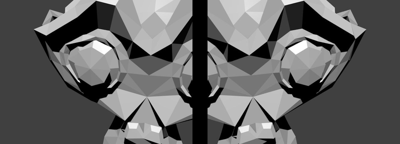
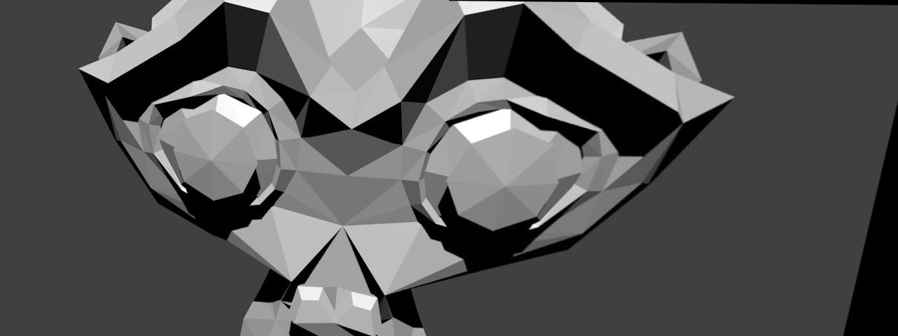
為了說明這一點，我們使用了 Blender（一款免費開源的 3D 計算機圖形軟體）來生成兩個相機檢視，它們之間只有旋轉變換。有關如何使用 Blender 獲取相機內參和相對於世界的 3x4 外參矩陣的更多資訊，請參見 11（還需要一個額外的變換才能獲得相機與物體座標系之間的變換）。

下圖顯示了 Suzanne 模型生成的兩個檢視，它們之間只有旋轉變換

已知關聯的相機位姿和內參，可以計算兩個檢視之間的相對旋轉

這裡，第二幅影像將相對於第一幅影像進行拼接。單應性可以使用上述公式計算

拼接操作很簡單